Network visualization

Installation

At first, fbnet library should be loaded. You can install fbnet and other useful packages with the following lines:

install.packages("fbnet") 
install.packages("pedtools") 
install.packages("mispitools") 
install.packages("forrel") 
library(fbnet)
library(pedtools)
library(mispitools)
library(forrel)

Setting up the pedigree

In this example, we use pedtools library for pedigree definition. Also, forrel R library provides the framework for genotype simulations, and mispitools library allows working with different reference allele frequencies databases.

Freqs <- lapply(getfreqs(Argentina), function(x) {x[x!=0]})
ped = linearPed(3)
ped = addChildren(ped, father =  1, mother =  2)
ped = pedtools::setMarkers(ped, locusAttributes = Freqs[1:3])
plot(ped, hatched = 8)

ped = profileSim(ped, N = 1, ids = 8, numCores = 10)[[1]]
#> Preparing parallelisation using 10 cores

So, the pedigree has the genetic information from the paternal grand uncle.

From pedtools to fbnet ped format

ConvertPedFormat function, from fbnet, allows working with pedtools pedigree format.

ped_fbnet <- convertPedformat(ped)

Analyzing the pedigree

Now we can put thing to work with fbnet.

pbn  <- initBN(ped_fbnet)
bnet <- buildBN(pbn,QP=7)
bn1  <- buildCPTs(bnet) 
resQ <- velim.bn(bn1,ordMethod="min_fill",verbose=FALSE)

Network visualization with igraph

For visualizing the network igraph package should be installed and loaded.

install.packages("igraph")
library(igraph)

plot(bnet[["DAG"]], layout=layout_with_fr, vertex.size=4,
     vertex.label.dist=0.7, vertex.label.color = "black", vertex.label.size = 20, vertex.color="black", edge.arrow.size=0.5)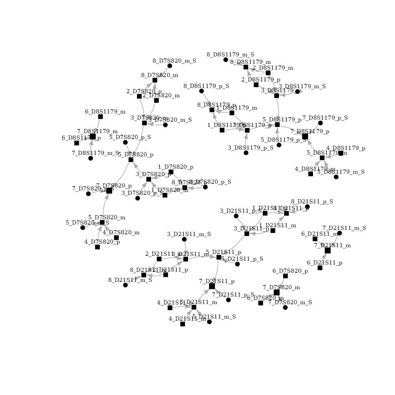

As previously explained, nodes represent alleles and edges conditional relationships. The node name represents: ID_marker_allele. Id is the individual number, marker is the name of the genetic marker, allele could be paternal (p) or maternal (m). Due to the complexity of the network, an iterative visualization could be a better option.

Network visualization with networkD3

First, for iterative network visualization networkD3 must be installed as follows:

install.packages("networkD3")
library(networkD3)

simpleNetwork(as_long_data_frame(bnet[[“DAG”]]), Source = 5, Target = 17, nodeColour = “black”) ?simpleNetwork

Iterative network could be visualized as follows:

simpleNetwork(as_long_data_frame(bnet[["DAG"]]), Source = 5, Target = 17, nodeColour = "black")

?simpleNetwork